Package laplace
The laplace package facilitates the application of Laplace approximations for entire neural networks, subnetworks of neural networks, or just their last layer. The package enables posterior approximations, marginal-likelihood estimation, and various posterior predictive computations. The library documentation is available at https://aleximmer.github.io/Laplace.
There is also a corresponding paper, Laplace Redux — Effortless Bayesian Deep Learning, which introduces the library, provides an introduction to the Laplace approximation, reviews its use in deep learning, and empirically demonstrates its versatility and competitiveness. Please consider referring to the paper when using our library:
@inproceedings{laplace2021,
  title={Laplace Redux--Effortless {B}ayesian Deep Learning},
  author={Erik Daxberger and Agustinus Kristiadi and Alexander Immer
          and Runa Eschenhagen and Matthias Bauer and Philipp Hennig},
  booktitle={{N}eur{IPS}},
  year={2021}
}
The code to reproduce the experiments in the paper is also publicly available; it provides examples of how to use our library for predictive uncertainty quantification, model selection, and continual learning.
[!IMPORTANT] As a user, one should not expect Laplace to work automatically. That is, one should experiment with different Laplace's options (hessian_factorization, prior precision tuning method, predictive method, backend, etc!). Try looking at various papers that use Laplace for references on how to set all those options depending on the applications/problems at hand.
Table of contents
- Setup
- Example usage
- Simple usage
- Marginal likelihood
- Laplace on LLM
- Subnetwork Laplace
- Serialization
- Structure
- Extendability
- When to use which backend?
- Contributing
- References
Setup
For full compatibility, install this package in a fresh virtual env.
We assume Python >= 3.9 since lower versions are (soon to be) deprecated.
PyTorch version 2.0 and up is also required for full compatibility.
To install laplace with pip, run the following:
pip install laplace-torch
For development purposes, clone the repository and then install:
# first install the build system:
pip install --upgrade pip wheel packaging

# then install the develop
pip install -e ".[all]"
Example usage
Simple usage
In the following example, a pre-trained model is loaded,
then the Laplace approximation is fit to the training data
(using a diagonal Hessian approximation over all parameters),
and the prior precision is optimized with cross-validation "gridsearch".
After that, the resulting LA is used for prediction with
the "probit" predictive for classification.
[!IMPORTANT] Laplace expects all data loaders, e.g.
train_loaderandval_loaderbelow, to be instances of PyTorchDataLoader. Each batch,next(iter(data_loader))must either be the standard(X, y)tensors or a dict-like object containing at least the keys specified indict_key_xanddict_key_yin Laplace's constructor.[!IMPORTANT] The total number of data points in all data loaders must be accessible via
len(train_loader.dataset).[!IMPORTANT] In
optimize_prior_precision, make sure to match the arguments with the ones you want to pass inla(x, …)during prediction.
from laplace import Laplace

# Pre-trained model
model = load_map_model()

# User-specified LA flavor
la = Laplace(model, "classification",
             subset_of_weights="all",
             hessian_structure="diag")
la.fit(train_loader)
la.optimize_prior_precision(
    method="gridsearch",
    pred_type="glm",
    link_approx="probit",
    val_loader=val_loader
)

# User-specified predictive approx.
pred = la(x, pred_type="glm", link_approx="probit")
Marginal likelihood
The marginal likelihood can be used for model selection [10] and is differentiable for continuous hyperparameters like the prior precision or observation noise. Here, we fit the library default, KFAC last-layer LA and differentiate the log marginal likelihood.
from laplace import Laplace

# Un- or pre-trained model
model = load_model()

# Default to recommended last-layer KFAC LA:
la = Laplace(model, likelihood="regression")
la.fit(train_loader)

# ML w.r.t. prior precision and observation noise
ml = la.log_marginal_likelihood(prior_prec, obs_noise)
ml.backward()
Laplace on LLM
[!TIP] This library also supports Huggingface models and parameter-efficient fine-tuning. See
examples/huggingface_examples.pyandexamples/huggingface_examples.mdfor the full exposition.
First, we need to wrap the pretrained model so that the forward method takes a
dict-like input. Note that when you iterate over a Huggingface dataloader,
this is what you get by default. Having a dict-like input is nice since different models
have different number of inputs (e.g. GPT-like LLMs only take input_ids, while BERT-like
ones take both input_ids and attention_mask, etc.). Inside this forward method you
can do your usual preprocessing like moving the tensor inputs into the correct device.
class MyGPT2(nn.Module):
    def __init__(self, tokenizer: PreTrainedTokenizer) -> None:
        super().__init__()
        config = GPT2Config.from_pretrained("gpt2")
        config.pad_token_id = tokenizer.pad_token_id
        config.num_labels = 2
        self.hf_model = GPT2ForSequenceClassification.from_pretrained(
            "gpt2", config=config
        )

    def forward(self, data: MutableMapping) -> torch.Tensor:
        device = next(self.parameters()).device
        input_ids = data["input_ids"].to(device)
        attn_mask = data["attention_mask"].to(device)
        output_dict = self.hf_model(input_ids=input_ids, attention_mask=attn_mask)
        return output_dict.logits
Then you can "select" which parameters of the LLM you want to apply the Laplace approximation
on, by switching off the gradients of the "unneeded" parameters.
For example, we can replicate a last-layer Laplace: (in actual practice, use Laplace(..., subset_of_weights='last_layer', ...) instead, though!)
model = MyGPT2(tokenizer)
model.eval()

# Enable grad only for the last layer
for p in model.hf_model.parameters():
    p.requires_grad = False
for p in model.hf_model.score.parameters():
    p.requires_grad = True

la = Laplace(
    model,
    likelihood="classification",
    # Will only hit the last-layer since it's the only one that is grad-enabled
    subset_of_weights="all",
    hessian_structure="diag",
)
la.fit(dataloader)
la.optimize_prior_precision()

test_data = next(iter(dataloader))
pred = la(test_data)
This is useful because we can apply the LA only on the parameter-efficient finetuning weights. E.g., we can fix the LLM itself, and apply the Laplace approximation only on the LoRA weights. Huggingface will automatically switch off the non-LoRA weights' gradients.
def get_lora_model():
    model = MyGPT2(tokenizer)  # Note we don't disable grad
    config = LoraConfig(
        r=4,
        lora_alpha=16,
        target_modules=["c_attn"],  # LoRA on the attention weights
        lora_dropout=0.1,
        bias="none",
    )
    lora_model = get_peft_model(model, config)
    return lora_model

lora_model = get_lora_model()

# Train it as usual here...

lora_model.eval()

lora_la = Laplace(
    lora_model,
    likelihood="classification",
    subset_of_weights="all",
    hessian_structure="diag",
    backend=AsdlGGN,
)

test_data = next(iter(dataloader))
lora_pred = lora_la(test_data)
Subnetwork Laplace
This example shows how to fit the Laplace approximation over only a subnetwork within a neural network (while keeping all other parameters fixed at their MAP estimates), as proposed in [11]. It also exemplifies different ways to specify the subnetwork to perform inference over.
from laplace import Laplace

# Pre-trained model
model = load_model()

# Examples of different ways to specify the subnetwork
# via indices of the vectorized model parameters
#
# Example 1: select the 128 parameters with the largest magnitude
from laplace.utils import LargestMagnitudeSubnetMask
subnetwork_mask = LargestMagnitudeSubnetMask(model, n_params_subnet=128)
subnetwork_indices = subnetwork_mask.select()

# Example 2: specify the layers that define the subnetwork
from laplace.utils import ModuleNameSubnetMask
subnetwork_mask = ModuleNameSubnetMask(model, module_names=["layer.1", "layer.3"])
subnetwork_mask.select()
subnetwork_indices = subnetwork_mask.indices

# Example 3: manually define the subnetwork via custom subnetwork indices
import torch
subnetwork_indices = torch.tensor([0, 4, 11, 42, 123, 2021])

# Define and fit subnetwork LA using the specified subnetwork indices
la = Laplace(model, "classification",
             subset_of_weights="subnetwork",
             hessian_structure="full",
             subnetwork_indices=subnetwork_indices)
la.fit(train_loader)
Serialization
As with plain torch, we support to ways to serialize data.
One is the familiar state_dict approach. Here you need to save and re-create
both model and Laplace(). Use this for long-term storage of models and
sharing of a fitted Laplace() instance.
# Save model and Laplace instance
torch.save(model.state_dict(), "model_state_dict.bin")
torch.save(la.state_dict(), "la_state_dict.bin")

# Load serialized data
model2 = MyModel(...)
model2.load_state_dict(torch.load("model_state_dict.bin"))
la2 = Laplace(model2, "classification",
              subset_of_weights="all",
              hessian_structure="diag")
la2.load_state_dict(torch.load("la_state_dict.bin"))
The second approach is to save the whole Laplace() object, including
self.model. This is less verbose and more convenient since you have the
trained model and the fitted Laplace() data stored in one place, but also comes with
some
drawbacks.
Use this for quick save-load cycles during experiments, say.
# Save Laplace, including la.model
torch.save(la, "la.pt")

# Load both
torch.load("la.pt")
Some Laplace variants such as LLLaplace might have trouble being serialized
using the default pickle module, which torch.save() and torch.load() use
(AttributeError: Can't pickle local object ...). In this case, the
dill package will come in handy.
import dill

torch.save(la, "la.pt", pickle_module=dill)
With both methods, you are free to switch devices, for instance when you trained on a GPU but want to run predictions on CPU. In this case, use
torch.load(..., map_location="cpu")
[!WARNING] Currently, this library always assumes that the model has an output tensor of shape
(batch_size, …, n_classes), so in the case of image outputs, you need to rearrange from NCHW to NHWC.
Structure
The laplace package consists of two main components:
- The subclasses of
laplace.BaseLaplacethat implement different sparsity structures: different subsets of weights ("all","subnetwork"and"last_layer") and different structures of the Hessian approximation ("full","kron","lowrank"and"diag"). This results in nine currently available options:FullLaplace,KronLaplace,DiagLaplace, the corresponding last-layer variationsFullLLLaplace,KronLLLaplace, andDiagLLLaplace(which are all subclasses oflaplace.LLLaplace),laplace.SubnetLaplace(which only supports"full"and"diag"Hessian approximations) andLowRankLaplace(which only supports inference over"all"weights). All of these can be conveniently accessed via thelaplace.Laplacefunction. - The backends in
laplace.curvaturewhich provide access to Hessian approximations of the corresponding sparsity structures, for example, the diagonal GGN.
Additionally, the package provides utilities for
decomposing a neural network into feature extractor and last layer for LLLaplace subclasses (laplace.utils.feature_extractor)
and
effectively dealing with Kronecker factors (laplace.utils.matrix).
Finally, the package implements several options to select/specify a subnetwork for SubnetLaplace (as subclasses of laplace.utils.subnetmask.SubnetMask).
Automatic subnetwork selection strategies include: uniformly at random (RandomSubnetMask), by largest parameter magnitudes (LargestMagnitudeSubnetMask), and by largest marginal parameter variances (LargestVarianceDiagLaplaceSubnetMask and LargestVarianceSWAGSubnetMask).
In addition to that, subnetworks can also be specified manually, by listing the names of either the model parameters (ParamNameSubnetMask) or modules (ModuleNameSubnetMask) to perform Laplace inference over.
Extendability
To extend the laplace package, new BaseLaplace subclasses can be designed, for example,
Laplace with a block-diagonal Hessian structure.
One can also implement custom subnetwork selection strategies as new subclasses of SubnetMask.
Alternatively, extending or integrating backends (subclasses of curvature.curvature) allows to provide different Hessian
approximations to the Laplace approximations.
For example, currently the curvature.CurvlinopsInterface based on Curvlinops and the native torch.func (previously known as functorch), curvature.BackPackInterface based on BackPACK and curvature.AsdlInterface based on ASDL are available.
When to use which backend
[!TIP] Each backend as its own caveat/behavior. The use the following to guide you picking the suitable backend, depending on you model & application.
- Small, simple MLP, or last-layer Laplace: Any backend should work well.
CurvlinopsGGNorCurvlinopsEFis recommended ifhessian_factorization = 'kron', but it's inefficient for other factorizations. - LLMs with PEFT (e.g. LoRA):
AsdlGGNandAsdlEFare recommended. - Continuous Bayesian optimization:
CurvlinopsGGN/EFandBackpackGGN/EFare recommended since they are the only ones supporting backprop over Jacobians.
[!CAUTION] The
curvlinopsbackends are inefficient for full and diagonal factorizations. Moreover, they're also inefficient for computing the Jacobians of large models since they rely ontorch.func.jacrevalongtorch.func.vmap! Finally,curvlinopsonly computes K-FAC (hessian_factorization = 'kron') fornn.Linearandnn.Conv2dmodules (including those inside larger modules like Attention).[!CAUTION] The
BackPackbackends are limited to models expressed asnn.Sequential. Also, they're not compatible with normalization layers.
Documentation
The documentation is available here or can be generated and/or viewed locally:
# assuming the repository was cloned
pip install -e ".[docs]"
# create docs and write to html
bash update_docs.sh
# .. or serve the docs directly
pdoc --http 0.0.0.0:8080 laplace --template-dir template
Contributing
Pull requests are very welcome. Please follow these guidelines:
- Install Laplace via
pip install -e ".[dev]"which will installruffand all requirements necessary to run the tests and build the docs. - Use ruff as autoformatter. Please refer to the following makefile and run it via
make ruff. Please note that the order ofruff check --fixandruff formatis important! - Also use ruff as linter. Please manually fix all linting errors/warnings before opening a pull request.
- Fully document your changes in the form of Python docstrings, typehinting, and (if applicable) code/markdown examples in the
./examplessubdirectory. - Provide as many test cases as possible. Make sure all test cases pass.
Issues, bug reports, and ideas are also very welcome!
References
This package relies on various improvements to the Laplace approximation for neural networks, which was originally due to MacKay [1]. Please consider citing the respective papers if you use any of their proposed methods via our laplace library.
- [1] MacKay, DJC. A Practical Bayesian Framework for Backpropagation Networks. Neural Computation 1992.
- [2] Gibbs, M. N. Bayesian Gaussian Processes for Regression and Classification. PhD Thesis 1997.
- [3] Snoek, J., Rippel, O., Swersky, K., Kiros, R., Satish, N., Sundaram, N., Patwary, M., Prabhat, M., Adams, R. Scalable Bayesian Optimization Using Deep Neural Networks. ICML 2015.
- [4] Ritter, H., Botev, A., Barber, D. A Scalable Laplace Approximation for Neural Networks. ICLR 2018.
- [5] Foong, A. Y., Li, Y., Hernández-Lobato, J. M., Turner, R. E. 'In-Between' Uncertainty in Bayesian Neural Networks. ICML UDL Workshop 2019.
- [6] Khan, M. E., Immer, A., Abedi, E., Korzepa, M. Approximate Inference Turns Deep Networks into Gaussian Processes. NeurIPS 2019.
- [7] Kristiadi, A., Hein, M., Hennig, P. Being Bayesian, Even Just a Bit, Fixes Overconfidence in ReLU Networks. ICML 2020.
- [8] Immer, A., Korzepa, M., Bauer, M. Improving predictions of Bayesian neural nets via local linearization. AISTATS 2021.
- [9] Sharma, A., Azizan, N., Pavone, M. Sketching Curvature for Efficient Out-of-Distribution Detection for Deep Neural Networks. UAI 2021.
- [10] Immer, A., Bauer, M., Fortuin, V., Rätsch, G., Khan, EM. Scalable Marginal Likelihood Estimation for Model Selection in Deep Learning. ICML 2021.
- [11] Daxberger, E., Nalisnick, E., Allingham, JU., Antorán, J., Hernández-Lobato, JM. Bayesian Deep Learning via Subnetwork Inference. ICML 2021.
Full example: Optimization of the marginal likelihood and prediction
Sinusoidal toy data
We show how the marginal likelihood can be used after training a MAP network on a simple sinusoidal regression task.
Subsequently, we use the optimized LA to predict which provides uncertainty on top of the MAP prediction.
We also show how the marglik_training() utility method can be used to jointly train the MAP and hyperparameters.
First, we set up the training data for the problem with observation noise \(\sigma=0.3\):
from laplace.baselaplace import FullLaplace
from laplace.curvature.backpack import BackPackGGN
import numpy as np
import torch

from laplace import Laplace, marglik_training

from helper.dataloaders import get_sinusoid_example
from helper.util import plot_regression

n_epochs = 1000
torch.manual_seed(711)
# sample toy data example
X_train, y_train, train_loader, X_test = get_sinusoid_example(sigma_noise=0.3)
Training a MAP
We now use pytorch to train a neural network with single hidden layer and Tanh activation.
The trained neural network will be our MAP estimate.
This is standard so nothing new here, yet:
# create and train MAP model
def get_model():
    torch.manual_seed(711)
    return torch.nn.Sequential(
        torch.nn.Linear(1, 50), torch.nn.Tanh(), torch.nn.Linear(50, 1)
    )
model = get_model()

criterion = torch.nn.MSELoss()
optimizer = torch.optim.Adam(model.parameters(), lr=1e-2)
for i in range(n_epochs):
    for X, y in train_loader:
        optimizer.zero_grad()
        loss = criterion(model(X), y)
        loss.backward()
        optimizer.step()
Fitting and optimizing the Laplace approximation using empirical Bayes
With the MAP-trained model at hand, we can estimate the prior precision and observation noise
using empirical Bayes after training.
The Laplace() method is called to construct a LA for "regression" with "all" weights.
As default Laplace() returns a Kronecker factored LA, we use "full" instead on this small example.
We fit the LA to the training data and initialize log_prior and log_sigma.
Using Adam, we minimize the negative log marginal likelihood for n_epochs.
la = Laplace(model, "regression", subset_of_weights="all", hessian_structure="full")
la.fit(train_loader)
log_prior, log_sigma = torch.ones(1, requires_grad=True), torch.ones(1, requires_grad=True)
hyper_optimizer = torch.optim.Adam([log_prior, log_sigma], lr=1e-1)
for i in range(n_epochs):
    hyper_optimizer.zero_grad()
    neg_marglik = - la.log_marginal_likelihood(log_prior.exp(), log_sigma.exp())
    neg_marglik.backward()
    hyper_optimizer.step()
The obtained observation noise is close to the ground truth with a value of \(\sigma \approx 0.28\) without the need for any validation data. The resulting prior precision is \(\delta \approx 0.10\).
Bayesian predictive
Here, we compare the MAP prediction to the obtained LA prediction. For LA, we have a closed-form predictive distribution on the output \(f\) which is a Gaussian \(\mathcal{N}(f(x;\theta_{MAP}), \mathbb{V}[f] + \sigma^2)\):
x = X_test.flatten().cpu().numpy()
f_mu, f_var = la(X_test)
f_mu = f_mu.squeeze().detach().cpu().numpy()
f_sigma = f_var.squeeze().sqrt().cpu().numpy()
pred_std = np.sqrt(f_sigma**2 + la.sigma_noise.item()**2)

plot_regression(X_train, y_train, x, f_mu, pred_std)
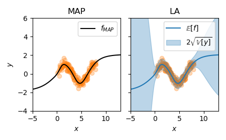
:align: center
In comparison to the MAP, the predictive shows useful uncertainties. When our MAP is over or underfit, the Laplace approximation cannot fix this anymore. In this case, joint optimization of MAP and marginal likelihood can be useful.
Jointly optimize MAP and hyperparameters using online empirical Bayes
We provide a utility method marglik_training() that implements the algorithm proposed in [1].
The method optimizes the neural network and the hyperparameters in an interleaved way
and returns an optimally regularized LA.
Below, we use this method and plot the corresponding predictive uncertainties again:
model = get_model()
la, model, margliks, losses = marglik_training(
    model=model, train_loader=train_loader, likelihood="regression",
    hessian_structure="full", backend=BackPackGGN, n_epochs=n_epochs,
    optimizer_kwargs={"lr": 1e-2}, prior_structure="scalar"
)

f_mu, f_var = la(X_test)
f_mu = f_mu.squeeze().detach().cpu().numpy()
f_sigma = f_var.squeeze().sqrt().cpu().numpy()
pred_std = np.sqrt(f_sigma**2 + la.sigma_noise.item()**2)

plot_regression(X_train, y_train, x, f_mu, pred_std)
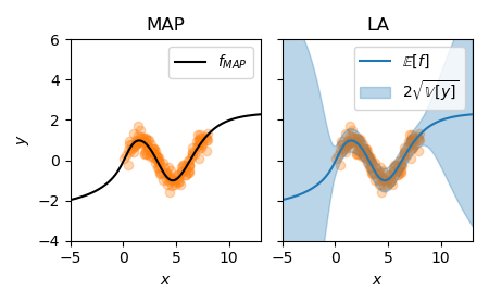
:align: center
Full example: post-hoc Laplace on a large image classifier
An advantage of the Laplace approximation over variational Bayes and Markov Chain Monte Carlo methods is its post-hoc nature. That means we can apply LA on (almost) any pre-trained neural network. In this example, we will see how we can apply the last-layer LA on a deep WideResNet model, trained on CIFAR-10.
Data loading
First, let us load the CIFAR-10 dataset. The helper scripts for CIFAR-10 and WideResNet are available in the examples/helper directory in the main repository.
import torch
import torch.distributions as dists
import numpy as np
import helper.wideresnet as wrn
import helper.dataloaders as dl
from helper import util
from netcal.metrics import ECE

from laplace import Laplace


np.random.seed(7777)
torch.manual_seed(7777)
torch.backends.cudnn.deterministic = True
torch.backends.cudnn.benchmark = True

train_loader = dl.CIFAR10(train=True)
test_loader = dl.CIFAR10(train=False)
targets = torch.cat([y for x, y in test_loader], dim=0).numpy()
Load a pre-trained model
Next, we will load a pre-trained WideResNet-16-4 model. Note that a GPU with CUDA support is needed for this example.
# The model is a standard WideResNet 16-4
# Taken as is from https://github.com/hendrycks/outlier-exposure
model = wrn.WideResNet(16, 4, num_classes=10).cuda().eval()

util.download_pretrained_model()
model.load_state_dict(torch.load("./temp/CIFAR10_plain.pt"))
To simplify the downstream tasks, we will use the following helper function to make predictions. It simply iterates through all minibatches and obtains the predictive probabilities of the CIFAR-10 classes.
@torch.no_grad()
def predict(dataloader, model, laplace=False):
    py = []

    for x, _ in dataloader:
        if laplace:
            py.append(model(x.cuda()))
        else:
            py.append(torch.softmax(model(x.cuda()), dim=-1))

    return torch.cat(py).cpu().numpy()
The calibration of MAP
We are now ready to see how calibrated is the model. The metrics we use are the expected calibration error (ECE, Naeni et al., AAAI 2015) and the negative (Categorical) log-likelihood. Note that lower values are better for both these metrics.
First, let us inspect the MAP model. We shall use the netcal library to easily compute the ECE.
probs_map = predict(test_loader, model, laplace=False)
acc_map = (probs_map.argmax(-1) == targets).float().mean()
ece_map = ECE(bins=15).measure(probs_map.numpy(), targets.numpy())
nll_map = -dists.Categorical(probs_map).log_prob(targets).mean()

print(f"[MAP] Acc.: {acc_map:.1%}; ECE: {ece_map:.1%}; NLL: {nll_map:.3}")
Running this snippet, we would get:
[MAP] Acc.: 94.8%; ECE: 2.0%; NLL: 0.172
The calibration of Laplace
Now we inspect the benefit of the LA. Let us apply the simple last-layer LA model, and optimize the prior precision hyperparameter using a post-hoc marginal likelihood maximization.
# Laplace
la = Laplace(model, "classification",
             subset_of_weights="last_layer",
             hessian_structure="kron")
la.fit(train_loader)
la.optimize_prior_precision(method="marglik")
Then, we are ready to see how well does LA improves the calibration of the MAP model:
probs_laplace = predict(test_loader, la, laplace=True)
acc_laplace = (probs_laplace.argmax(-1) == targets).float().mean()
ece_laplace = ECE(bins=15).measure(probs_laplace.numpy(), targets.numpy())
nll_laplace = -dists.Categorical(probs_laplace).log_prob(targets).mean()

print(f"[Laplace] Acc.: {acc_laplace:.1%}; ECE: {ece_laplace:.1%}; NLL: {nll_laplace:.3}")
Running this snippet, we obtain:
[Laplace] Acc.: 94.8%; ECE: 0.8%; NLL: 0.157
Notice that the last-layer LA does not do any harm to the accuracy, yet it improves the calibration of the MAP model substantially.
Full Example: Applying Laplace on a Huggingface LLM model
In this example, we will see how to apply Laplace on a GPT2 Huggingface (HF) model.
Laplace only has lightweight requirements for this; namely that the model's forward
method must only take a single dict-like object (dict, UserDict, or in general,
collections.abc.MutableMapping). This is entirely compatible with HF since HF's
data loaders are assumed to emit an object derived from UserDict. However, you
need to ensure this yourself — you need to wrap the standard HF model to conform
to that requirement. Also, you need to e.g. do torch.to(device) inside the
said forward method.
Let's start with as usual with importing stuff.
from collections.abc import MutableMapping
from collections import UserDict
import numpy
import torch
from torch import nn
import torch.utils.data as data_utils

from laplace import Laplace

import logging
import warnings

logging.basicConfig(level="ERROR")
warnings.filterwarnings("ignore")

from transformers import ( # noqa: E402
    GPT2Config,
    GPT2ForSequenceClassification,
    GPT2Tokenizer,
    DataCollatorWithPadding,
    PreTrainedTokenizer,
)
from peft import LoraConfig, get_peft_model # noqa: E402
from datasets import Dataset # noqa: E402

# make deterministic

torch.manual_seed(0)
numpy.random.seed(0)
Next, we create a toy dataset. You can use any HF datasets or your own, of course.
tokenizer = GPT2Tokenizer.from_pretrained("gpt2")
tokenizer.pad_token_id = tokenizer.eos_token_id

data = [
    {"text": "Today is hot, but I will manage!!!!", "label": 1},
    {"text": "Tomorrow is cold", "label": 0},
    {"text": "Carpe diem", "label": 1},
    {"text": "Tempus fugit", "label": 1},
]
dataset = Dataset.from_list(data)

def tokenize(row):
    return tokenizer(row["text"])

dataset = dataset.map(tokenize, remove_columns=["text"])
dataset.set_format(type="torch", columns=["input_ids", "attention_mask", "label"])
dataloader = data_utils.DataLoader(
    dataset, batch_size=100, collate_fn=DataCollatorWithPadding(tokenizer)
)

data = next(iter(dataloader))
print(
    f"Huggingface data defaults to UserDict, which is a MutableMapping? {isinstance(data, UserDict)}"
)
for k, v in data.items():
    print(k, v.shape)
This is the output:
Huggingface data defaults to UserDict, which is a MutableMapping? True
input_ids torch.Size([4, 9])
attention_mask torch.Size([4, 9])
labels torch.Size([4])
Laplace on a subset of an LLM's weights
Now, let's do the main "meat" of this example: Wrapping the HF model into a model that is
compatible with Laplace. Notice that this wrapper just wraps the HF model and nothing else.
Notice also we do inputs.to(device) inside self.forward().
class MyGPT2(nn.Module):
    """
    Huggingface LLM wrapper.

    Args:
        tokenizer: The tokenizer used for preprocessing the text data. Needed
            since the model needs to know the padding token id.
    """

    def __init__(self, tokenizer: PreTrainedTokenizer) -> None:
        super().__init__()
        config = GPT2Config.from_pretrained("gpt2")
        config.pad_token_id = tokenizer.pad_token_id
        config.num_labels = 2
        self.hf_model = GPT2ForSequenceClassification.from_pretrained(
            "gpt2", config=config
        )

    def forward(self, data: MutableMapping) -> torch.Tensor:
        """
        Custom forward function. Handles things like moving the
        input tensor to the correct device inside.

        Args:
            data: A dict-like data structure with `input_ids` inside.
                This is the default data structure assumed by Huggingface
                dataloaders.

        Returns:
            logits: An `(batch_size, n_classes)`-sized tensor of logits.
        """
        device = next(self.parameters()).device
        input_ids = data["input_ids"].to(device)
        attn_mask = data["attention_mask"].to(device)
        output_dict = self.hf_model(input_ids=input_ids, attention_mask=attn_mask)
        return output_dict.logits

model = MyGPT2(tokenizer)
Now, let's apply Laplace. Let's do a last-layer Laplace first.
Notice that we add
an argument feature_reduction there. This is because Huggingface models reduce the
logits and not the features.
model = MyGPT2(tokenizer)
model.eval()

la = Laplace(
    model,
    likelihood="classification",
    subset_of_weights="last_layer",
    hessian_structure="full",
    # This must reflect faithfully the reduction technique used in the model
    # Otherwise, correctness is not guaranteed
    feature_reduction="pick_last",
)
la.fit(dataloader)
la.optimize_prior_precision()

X_test = next(iter(dataloader))
print(f"[Last-layer Laplace] The predictive tensor is of shape: {la(X_test).shape}.")
Here's the output:
[Last-layer Laplace] The predictive tensor is of shape: torch.Size([4, 2]).
Subnetwork Laplace
Also, we can do the same thing by switching off the gradients of all layers except the
top layer. Laplace will automatically only compute the Hessian (and Jacobians) of the
parameters in which requires_grad is True.
Notice that you can "mix-and-match" this gradient switching. You can do a subnetwork Laplace easily by doing so!
model.eval()

# Enable grad only for the last layer

for p in model.hf_model.parameters():
    p.requires_grad = False

for p in model.hf_model.score.parameters():
    p.requires_grad = True

la = Laplace(
    model,
    # Will only hit the last-layer since it's the only one that is grad-enabled
    likelihood="classification",
    subset_of_weights="all",
    hessian_structure="diag",
)
la.fit(dataloader)
la.optimize_prior_precision()

X_test = next(iter(dataloader))
print(f"[Subnetwork Laplace] The predictive tensor is of shape: {la(X_test).shape}.")
Here are the outputs to validate that Laplace works:
[Subnetwork Laplace] The predictive tensor is of shape: torch.Size([4, 2]).
Full Laplace on LoRA parameters only
Of course, you can also apply Laplace on the parameter-efficient fine tuning weights (like LoRA).
To do this, simply extend your LLM with LoRA, using HF's peft library, and apply Laplace as
usual. Note that peft automatically switches off the non-LoRA weights.
def get_lora_model():
    model = MyGPT2(tokenizer) # Note we don't disable grad
    config = LoraConfig(
        r=4,
        lora_alpha=16,
        target_modules=["c_attn"], # LoRA on the attention weights
        lora_dropout=0.1,
        bias="none",
    )
    lora_model = get_peft_model(model, config)
    return lora_model

lora_model = get_lora_model()

# Train it as usual

lora_model.eval()

lora_la = Laplace(
    lora_model,
    likelihood="classification",
    subset_of_weights="all",
    hessian_structure="kron",
)
lora_la.fit(dataloader)

X_test = next(iter(dataloader))
print(f"[LoRA-LLM] The predictive tensor is of shape: {lora_la(X_test).shape}.")
Here is the output, as expected:
[LoRA-LLM] The predictive tensor is of shape: torch.Size([4, 2]).
As a final note, the dict-like input requirement of Laplace is very flexible. It can essentially be applicable to any tasks and any models. You just need to wrap the said model and make sure that your data loaders emit dict-like objects, where the input tensors are the dicts' values.
Caveats
Currently, diagonal EF with the Curvlinops backend is unsupported for dict-based inputs.
This is because we use torch.func's vmap to compute the diag-EF, and it only accepts
tensor input in the model's forward.
See this issue.
So, if you can write down your Huggingface model's forward to accept only a single tensor,
this is much preferable.
For instance, in the case of causal LLM like GPTs, only input_ids
tensor is necessary.
Then, any backend and any hessian factorization can be used in this case.
Otherwise, if you must use dict-based inputs, choose the following backends:
CurvlinopsGGNforhessian_factorization = {"kron", "diag"}CurvlinopsEFforhessian_factorization = {"kron"}AsdlGGNforhessian_factorization = {"kron", "diag"}AsdlEFforhessian_factorization = {"kron", "diag"}
Full Example: Bayesian Bradley-Terry Reward Modeling
The laplace-torch library can also be used to "Bayesianize" a pretrained Bradley-Terry
reward model, popular in large language models. See http://arxiv.org/abs/2009.01325
for a primer in reward modeling.
First order of business, let's define our comparison dataset. We will use the datasets
library from Huggingface to handle the data.
import numpy as np
import torch
from torch import nn, optim
from torch.nn import functional as F
import torch.utils.data as data_utils

from datasets import Dataset

from laplace import Laplace

import logging
import warnings

logging.basicConfig(level="ERROR")
warnings.filterwarnings("ignore")

# make deterministic
torch.manual_seed(0)
np.random.seed(0)


# Pairwise comparison dataset. The label indicates which `x0` or `x1` is preferred.
data_dict = [
    {
        "x0": torch.randn(3),
        "x1": torch.randn(3),
        "label": torch.randint(2, size=(1,)).item(),
    }
    for _ in range(10)
]
dataset = Dataset.from_list(data_dict)
Now, let's define the reward model. During training, it assumes that x is a tensor
of shape (batch_size, 2, dim), which is a concatenation of x0 and x1 above.
The second dimension of size 2 is preserved through the forward pass, resulting in
a logit tensor of shape (batch_size, 2) (the network itself is single-output).
Then, the standard cross-entropy loss is applied.
Note that this requirement is quite weak and can covers general cases. However, if you prefer to use the dict-like inputs as in Huggingface LLM models, this can also be done. Simply combine what you have learned from this example with the Huggingface LLM example provided in this library.
During testing, this model behaves like a standard single-output regression model.
class SimpleRewardModel(nn.Module):
    """A simple reward model, compatible with the Bradley-Terry likelihood.
    """

    def __init__(self):
        super().__init__()
        self.net = nn.Sequential(nn.Linear(3, 100), nn.ReLU(), nn.Linear(100, 1))

    def forward(self, x):
        """Args:
            x: torch.Tensor
                If training == True then shape (batch_size, 2, dim)
                Else shape (batch_size, dim)

        Returns:
            logits: torch.Tensor
                If training then shape (batch_size, 2)
                Else shape (batch_size, 1)
        """
        if len(x.shape) == 3:
            batch_size, _, dim = x.shape

            # Flatten to (batch_size*2, dim)
            flat_x = x.reshape(-1, dim)

            # Forward
            flat_logits = self.net(flat_x)  # (batch_size*2, 1)

            # Reshape back to (batch_size, 2)
            return flat_logits.reshape(batch_size, 2)
        else:
            logits = self.net(x)  # (batch_size, 1)
            return logits
To fulfill the 3D tensor requirement, we need to preprocess the dict-based dataset.
# Preprocess to coalesce x0 and x1 into a single array/tensor
def append_x0_x1(row):
    # The tensor values above are automatically casted as lists by `Dataset`
    row["x"] = np.stack([row["x0"], row["x1"]])  # (2, dim)
    return row


tensor_dataset = dataset.map(append_x0_x1, remove_columns=["x0", "x1"])
tensor_dataset.set_format(type="torch", columns=["x", "label"])
tensor_dataloader = data_utils.DataLoader(
    data_utils.TensorDataset(tensor_dataset["x"], tensor_dataset["label"]), batch_size=3
)
Then, we can train as usual using the cross entropy loss.
reward_model = SimpleRewardModel()
opt = optim.AdamW(reward_model.parameters(), weight_decay=1e-3)

# Train as usual
for epoch in range(10):
    for x, y in tensor_dataloader:
        opt.zero_grad()
        out = reward_model(x)
        loss = F.cross_entropy(out, y)
        loss.backward()
        opt.step()
Applying Laplace to this model is a breeze. Simply state that the likelihood is reward_modeling.
# Laplace !!! Notice the likelihood !!!
reward_model.eval()
la = Laplace(reward_model, likelihood="reward_modeling", subset_of_weights="all")
la.fit(tensor_dataloader)
la.optimize_prior_precision()
As we can see, during prediction, even though we train & fit Laplace using the cross entropy loss (i.e. classification), in test time, the model behaves like a regression model. So, you don't get probability vectors as outputs. Instead, you get two tensors containing the predictive means and predictive variance.
x_test = torch.randn(5, 3)
pred_mean, pred_var = la(x_test)
print(
    f"Input shape {tuple(x_test.shape)}, predictive mean of shape "
    + f"{tuple(pred_mean.shape)}, predictive covariance of shape "
    + f"{tuple(pred_var.shape)}"
)
Here's the output:
Input shape (5, 3), predictive mean of shape (5, 1), predictive covariance of shape (5, 1, 1)
Sub-modules
laplace.baselaplacelaplace.curvaturelaplace.laplacelaplace.lllaplacelaplace.subnetlaplacelaplace.utils
Functions
def Laplace(model: torch.nn.Module, likelihood: Likelihood | str, subset_of_weights: SubsetOfWeights | str = SubsetOfWeights.LAST_LAYER, hessian_structure: HessianStructure | str = HessianStructure.KRON, *args, **kwargs) ‑> ParametricLaplace-
Simplified Laplace access using strings instead of different classes.
Parameters
model:torch.nn.Modulelikelihood:Likelihoodorstr in {'classification', 'regression'}subset_of_weights:SubsetofWeightsor{'last_layer', 'subnetwork', 'all'}, default=SubsetOfWeights.LAST_LAYER- subset of weights to consider for inference
hessian_structure:HessianStructureorstr in {'diag', 'kron', 'full', 'lowrank'}, default=HessianStructure.KRON- structure of the Hessian approximation
Returns
laplace:ParametricLaplace- chosen subclass of ParametricLaplace instantiated with additional arguments
def marglik_training(model: torch.nn.Module, train_loader: DataLoader, likelihood: Likelihood | str = Likelihood.CLASSIFICATION, hessian_structure: HessianStructure | str = HessianStructure.KRON, backend: Type[CurvatureInterface] = laplace.curvature.asdl.AsdlGGN, optimizer_cls: Type[Optimizer] = torch.optim.adam.Adam, optimizer_kwargs: dict | None = None, scheduler_cls: Type[LRScheduler] | None = None, scheduler_kwargs: dict | None = None, n_epochs: int = 300, lr_hyp: float = 0.1, prior_structure: PriorStructure | str = PriorStructure.LAYERWISE, n_epochs_burnin: int = 0, n_hypersteps: int = 10, marglik_frequency: int = 1, prior_prec_init: float = 1.0, sigma_noise_init: float = 1.0, temperature: float = 1.0, fix_sigma_noise: bool = False, progress_bar: bool = False, enable_backprop: bool = False, dict_key_x: str = 'input_ids', dict_key_y: str = 'labels') ‑> tuple[BaseLaplace, nn.Module, list[Number], list[Number]]-
Marginal-likelihood based training (Algorithm 1 in [1]). Optimize model parameters and hyperparameters jointly. Model parameters are optimized to minimize negative log joint (train loss) while hyperparameters minimize negative log marginal likelihood.
This method replaces standard neural network training and adds hyperparameter optimization to the procedure.
The settings of standard training can be controlled by passing
train_loader,optimizer_cls,optimizer_kwargs,scheduler_cls,scheduler_kwargs, andn_epochs. Themodelshould return logits, i.e., no softmax should be applied. Withlikelihood=Likelihood.CLASSIFICATIONorLikelihood.REGRESSION, one can choose between categorical likelihood (CrossEntropyLoss) and Gaussian likelihood (MSELoss).As in [1], we optimize prior precision and, for regression, observation noise using the marginal likelihood. The prior precision structure can be chosen as
'scalar','layerwise', or'diagonal'.'layerwise'is a good default and available to all Laplace approximations.lr_hypis the step size of the Adam hyperparameter optimizer,n_hyperstepscontrols the number of steps for each estimated marginal likelihood,n_epochs_burnincontrols how many epochs to skip marginal likelihood estimation,marglik_frequencycontrols how often to estimate the marginal likelihood (default of 1 re-estimates after every epoch, 5 would estimate every 5-th epoch).References
[1] Immer, A., Bauer, M., Fortuin, V., Rätsch, G., Khan, EM. Scalable Marginal Likelihood Estimation for Model Selection in Deep Learning. ICML 2021.
Parameters
model:torch.nn.Module- torch neural network model (needs to comply with Backend choice)
train_loader:DataLoader- pytorch dataloader that implements
len(train_loader.dataset)to obtain number of data points likelihood:str, default=Likelihood.CLASSIFICATION- Likelihood.CLASSIFICATION or Likelihood.REGRESSION
hessian_structure:{'diag', 'kron', 'full'}, default='kron'- structure of the Hessian approximation
backend:Backend, default=AsdlGGN- Curvature subclass, e.g. AsdlGGN/AsdlEF or BackPackGGN/BackPackEF
optimizer_cls:torch.optim.Optimizer, default=Adam- optimizer to use for optimizing the neural network parameters togeth with
train_loader optimizer_kwargs:dict, default=None- keyword arguments for
optimizer_cls, for example to change learning rate or momentum scheduler_cls:torch.optim.lr_scheduler._LRScheduler, default=None- optionally, a scheduler to use on the learning rate of the optimizer.
scheduler.step()is called after every batch of the standard training. scheduler_kwargs:dict, default=None- keyword arguments for
scheduler_cls, e.g.lr_minfor CosineAnnealingLR n_epochs:int, default=300- number of epochs to train for
lr_hyp:float, default=0.1- Adam learning rate for hyperparameters
prior_structure:str, default='layerwise'- structure of the prior. one of
['scalar', 'layerwise', 'diag'] n_epochs_burnin:int default=0- how many epochs to train without estimating and differentiating marglik
n_hypersteps:int, default=10- how many steps to take on the hyperparameters when marglik is estimated
marglik_frequency:int- how often to estimate (and differentiate) the marginal likelihood
marglik_frequency=1would be every epoch,marglik_frequency=5would be every 5 epochs. prior_prec_init:float, default=1.0- initial prior precision
sigma_noise_init:float, default=1.0- initial observation noise (for regression only)
temperature:float, default=1.0- factor for the likelihood for 'overcounting' data. Might be required for data augmentation.
fix_sigma_noise:bool, default=False- if False, optimize observation noise via marglik otherwise use
sigma_noise_initthroughout. Only works for regression. progress_bar:bool, default=False- whether to show a progress bar (updated per epoch) or not
enable_backprop:bool, default=False- make the returned Laplace instance backpropable—useful for e.g. Bayesian optimization.
dict_key_x:str, default='input_ids'- The dictionary key under which the input tensor
xis stored. Only has effect when the model takes aMutableMappingas the input. Useful for Huggingface LLM models. dict_key_y:str, default='labels'- The dictionary key under which the target tensor
yis stored. Only has effect when the model takes aMutableMappingas the input. Useful for Huggingface LLM models.
Returns
lap:laplace.laplace- fit Laplace approximation with the best obtained marginal likelihood during training
model:torch.nn.Module- corresponding model with the MAP parameters
margliks:list- list of marginal likelihoods obtained during training (to monitor convergence)
losses:list- list of losses (log joints) obtained during training (to monitor convergence)
Classes
class BaseLaplace (model: nn.Module, likelihood: Likelihood | str, sigma_noise: float | torch.Tensor = 1.0, prior_precision: float | torch.Tensor = 1.0, prior_mean: float | torch.Tensor = 0.0, temperature: float = 1.0, enable_backprop: bool = False, dict_key_x: str = 'input_ids', dict_key_y: str = 'labels', backend: type[CurvatureInterface] | None = None, backend_kwargs: dict[str, Any] | None = None, asdl_fisher_kwargs: dict[str, Any] | None = None)-
Baseclass for all Laplace approximations in this library.
Parameters
model:torch.nn.Modulelikelihood:Likelihoodorstr in {'classification', 'regression', 'reward_modeling'}- determines the log likelihood Hessian approximation.
In the case of 'reward_modeling', it fits Laplace using the classification likelihood,
then does prediction as in regression likelihood. The model needs to be defined accordingly:
The forward pass during training takes
x.shape == (batch_size, 2, dim)withy.shape = (batch_size,). Meanwhile, during evaluationx.shape == (batch_size, dim). Note that 'reward_modeling' only supportsKronLaplaceandDiagLaplace. sigma_noise:torch.Tensororfloat, default=1- observation noise for the regression setting; must be 1 for classification
prior_precision:torch.Tensororfloat, default=1- prior precision of a Gaussian prior (= weight decay); can be scalar, per-layer, or diagonal in the most general case
prior_mean:torch.Tensororfloat, default=0- prior mean of a Gaussian prior, useful for continual learning
temperature:float, default=1- temperature of the likelihood; lower temperature leads to more concentrated posterior and vice versa.
enable_backprop:bool, default=False- whether to enable backprop to the input
xthrough the Laplace predictive. Useful for e.g. Bayesian optimization. dict_key_x:str, default='input_ids'- The dictionary key under which the input tensor
xis stored. Only has effect when the model takes aMutableMappingas the input. Useful for Huggingface LLM models. dict_key_y:str, default='labels'- The dictionary key under which the target tensor
yis stored. Only has effect when the model takes aMutableMappingas the input. Useful for Huggingface LLM models. backend:subclassesofCurvatureInterface- backend for access to curvature/Hessian approximations. Defaults to CurvlinopsGGN if None.
backend_kwargs:dict, default=None- arguments passed to the backend on initialization, for example to set the number of MC samples for stochastic approximations.
asdl_fisher_kwargs:dict, default=None- arguments passed to the ASDL backend specifically on initialization.
Subclasses
- laplace.baselaplace.FunctionalLaplace
- ParametricLaplace
Instance variables
var backend : CurvatureInterfacevar log_likelihood : torch.Tensor-
Compute log likelihood on the training data after
.fit()has been called. The log likelihood is computed on-demand based on the loss and, for example, the observation noise which makes it differentiable in the latter for iterative updates.Returns
log_likelihood:torch.Tensor
var prior_precision_diag : torch.Tensor-
Obtain the diagonal prior precision p_0 constructed from either a scalar, layer-wise, or diagonal prior precision.
Returns
prior_precision_diag:torch.Tensor
var prior_mean : torch.Tensorvar prior_precision : torch.Tensorvar sigma_noise : torch.Tensor
Methods
def fit(self, train_loader: DataLoader) ‑> Nonedef log_marginal_likelihood(self, prior_precision: torch.Tensor | None = None, sigma_noise: torch.Tensor | None = None) ‑> torch.Tensordef predictive(self, x: torch.Tensor, pred_type: PredType | str, link_approx: LinkApprox | str, n_samples: int) ‑> torch.Tensor | tuple[torch.Tensor, torch.Tensor]def optimize_prior_precision(self, pred_type: PredType | str, method: TuningMethod | str = TuningMethod.MARGLIK, n_steps: int = 100, lr: float = 0.1, init_prior_prec: float | torch.Tensor = 1.0, prior_structure: PriorStructure | str = PriorStructure.DIAG, val_loader: DataLoader | None = None, loss: torchmetrics.Metric | Callable[[torch.Tensor], torch.Tensor | float] | None = None, log_prior_prec_min: float = -4, log_prior_prec_max: float = 4, grid_size: int = 100, link_approx: LinkApprox | str = LinkApprox.PROBIT, n_samples: int = 100, verbose: bool = False, progress_bar: bool = False) ‑> None-
Optimize the prior precision post-hoc using the
methodspecified by the user.Parameters
pred_type:PredTypeorstr in {'glm', 'nn'}- type of posterior predictive, linearized GLM predictive or neural network sampling predictiv. The GLM predictive is consistent with the curvature approximations used here.
method:TuningMethodorstr in {'marglik', 'gridsearch'}, default=PredType.MARGLIK- specifies how the prior precision should be optimized.
n_steps:int, default=100- the number of gradient descent steps to take.
lr:float, default=1e-1- the learning rate to use for gradient descent.
init_prior_prec:floatortensor, default=1.0- initial prior precision before the first optimization step.
prior_structure:PriorStructureorstr in {'scalar', 'layerwise', 'diag'}, default=PriorStructure.SCALAR- if init_prior_prec is scalar, the prior precision is optimized with this structure. otherwise, the structure of init_prior_prec is maintained.
val_loader:torch.data.utils.DataLoader, default=None- DataLoader for the validation set; each iterate is a training batch (X, y).
loss:callableortorchmetrics.Metric, default=None- loss function to use for CV. If callable, the loss is computed offline (memory intensive).
If torchmetrics.Metric, running loss is computed (efficient). The default
depends on the likelihood:
RunningNLLMetric()for classification and reward modeling, runningMeanSquaredError()for regression. log_prior_prec_min:float, default=-4- lower bound of gridsearch interval.
log_prior_prec_max:float, default=4- upper bound of gridsearch interval.
grid_size:int, default=100- number of values to consider inside the gridsearch interval.
link_approx:LinkApproxorstr in {'mc', 'probit', 'bridge'}, default=LinkApprox.PROBIT- how to approximate the classification link function for the
'glm'. Forpred_type='nn', only'mc'is possible. n_samples:int, default=100- number of samples for
link_approx='mc'. verbose:bool, default=False- if true, the optimized prior precision will be printed (can be a large tensor if the prior has a diagonal covariance).
progress_bar:bool, default=False- whether to show a progress bar; updated at every batch-Hessian computation.
Useful for very large model and large amount of data, esp. when
subset_of_weights='all'.
class ParametricLaplace (model: nn.Module, likelihood: Likelihood | str, sigma_noise: float | torch.Tensor = 1.0, prior_precision: float | torch.Tensor = 1.0, prior_mean: float | torch.Tensor = 0.0, temperature: float = 1.0, enable_backprop: bool = False, dict_key_x: str = 'inputs_id', dict_key_y: str = 'labels', backend: type[CurvatureInterface] | None = None, backend_kwargs: dict[str, Any] | None = None, asdl_fisher_kwargs: dict[str, Any] | None = None)-
Parametric Laplace class.
Subclasses need to specify how the Hessian approximation is initialized, how to add up curvature over training data, how to sample from the Laplace approximation, and how to compute the functional variance.
A Laplace approximation is represented by a MAP which is given by the
modelparameter and a posterior precision or covariance specifying a Gaussian distribution \mathcal{N}(\theta_{MAP}, P^{-1}). The goal of this class is to compute the posterior precision P which sums as P = \sum_{n=1}^N \nabla^2_\theta \log p(\mathcal{D}_n \mid \theta) \vert_{\theta_{MAP}} + \nabla^2_\theta \log p(\theta) \vert_{\theta_{MAP}}. Every subclass implements different approximations to the log likelihood Hessians, for example, a diagonal one. The prior is assumed to be Gaussian and therefore we have a simple form for \nabla^2_\theta \log p(\theta) \vert_{\theta_{MAP}} = P_0 . In particular, we assume a scalar, layer-wise, or diagonal prior precision so that in all cases P_0 = \textrm{diag}(p_0) and the structure of p_0 can be varied.Ancestors
Subclasses
Instance variables
var scatter : torch.Tensor-
Computes the scatter, a term of the log marginal likelihood that corresponds to L-2 regularization:
scatter= (\theta_{MAP} - \mu_0)^{T} P_0 (\theta_{MAP} - \mu_0) .Returns
scatter:torch.Tensor
var log_det_prior_precision : torch.Tensor-
Compute log determinant of the prior precision \log \det P_0
Returns
log_det:torch.Tensor
var log_det_posterior_precision : torch.Tensor-
Compute log determinant of the posterior precision \log \det P which depends on the subclasses structure used for the Hessian approximation.
Returns
log_det:torch.Tensor
var log_det_ratio : torch.Tensor-
Compute the log determinant ratio, a part of the log marginal likelihood. \log \frac{\det P}{\det P_0} = \log \det P - \log \det P_0
Returns
log_det_ratio:torch.Tensor
var posterior_precision : torch.Tensor-
Compute or return the posterior precision P.
Returns
posterior_prec:torch.Tensor
Methods
def fit(self, train_loader: DataLoader, override: bool = True, progress_bar: bool = False) ‑> None-
Fit the local Laplace approximation at the parameters of the model.
Parameters
train_loader:torch.data.utils.DataLoader- each iterate is a training batch, either
(X, y)tensors or a dict-like object containing keys as expressed byself.dict_key_xandself.dict_key_y.train_loader.datasetneeds to be set to access N, size of the data set. override:bool, default=True- whether to initialize H, loss, and n_data again; setting to False is useful for online learning settings to accumulate a sequential posterior approximation.
progress_bar:bool, default=False- whether to show a progress bar; updated at every batch-Hessian computation.
Useful for very large model and large amount of data, esp. when
subset_of_weights='all'.
def square_norm(self, value) ‑> torch.Tensor-
Compute the square norm under post. Precision with
value-self.meanas 𝛥: \Delta^ op P \Delta Returns
square_form
def log_prob(self, value: torch.Tensor, normalized: bool = True) ‑> torch.Tensor-
Compute the log probability under the (current) Laplace approximation.
Parameters
value:torch.Tensornormalized:bool, default=True- whether to return log of a properly normalized Gaussian or just the
terms that depend on
value.
Returns
log_prob:torch.Tensor
def log_marginal_likelihood(self, prior_precision: torch.Tensor | None = None, sigma_noise: torch.Tensor | None = None) ‑> torch.Tensor-
Compute the Laplace approximation to the log marginal likelihood subject to specific Hessian approximations that subclasses implement. Requires that the Laplace approximation has been fit before. The resulting torch.Tensor is differentiable in
prior_precisionandsigma_noiseif these have gradients enabled. By passingprior_precisionorsigma_noise, the current value is overwritten. This is useful for iterating on the log marginal likelihood.Parameters
prior_precision:torch.Tensor, optional- prior precision if should be changed from current
prior_precisionvalue sigma_noise:torch.Tensor, optional- observation noise standard deviation if should be changed
Returns
log_marglik:torch.Tensor
def predictive_samples(self, x: torch.Tensor | MutableMapping[str, torch.Tensor | Any], pred_type: PredType | str = PredType.GLM, n_samples: int = 100, diagonal_output: bool = False, generator: torch.Generator | None = None) ‑> torch.Tensor-
Sample from the posterior predictive on input data
x. Can be used, for example, for Thompson sampling.Parameters
x:torch.TensororMutableMapping- input data
(batch_size, input_shape) pred_type:{'glm', 'nn'}, default='glm'- type of posterior predictive, linearized GLM predictive or neural network sampling predictive. The GLM predictive is consistent with the curvature approximations used here.
n_samples:int- number of samples
diagonal_output:bool- whether to use a diagonalized glm posterior predictive on the outputs.
Only applies when
pred_type='glm'. generator:torch.Generator, optional- random number generator to control the samples (if sampling used)
Returns
samples:torch.Tensor- samples
(n_samples, batch_size, output_shape)
def functional_variance(self, Js: torch.Tensor) ‑> torch.Tensor-
Compute functional variance for the
'glm'predictive:f_var[i] = Js[i] @ P.inv() @ Js[i].T, which is a output x output predictive covariance matrix. Mathematically, we have for a single Jacobian \mathcal{J} = \nabla_\theta f(x;\theta)\vert_{\theta_{MAP}} the output covariance matrix \mathcal{J} P^{-1} \mathcal{J}^T .Parameters
Js:torch.Tensor- Jacobians of model output wrt parameters
(batch, outputs, parameters)
Returns
f_var:torch.Tensor- output covariance
(batch, outputs, outputs)
def functional_covariance(self, Js: torch.Tensor) ‑> torch.Tensor-
Compute functional covariance for the
'glm'predictive:f_cov = Js @ P.inv() @ Js.T, which is a batchoutput x batchoutput predictive covariance matrix.This emulates the GP posterior covariance N([f(x1), …,f(xm)], Cov[f(x1), …, f(xm)]). Useful for joint predictions, such as in batched Bayesian optimization.
Parameters
Js:torch.Tensor- Jacobians of model output wrt parameters
(batch*outputs, parameters)
Returns
f_cov:torch.Tensor- output covariance
(batch*outputs, batch*outputs)
def sample(self, n_samples: int = 100, generator: torch.Generator | None = None) ‑> torch.Tensor-
Sample from the Laplace posterior approximation, i.e., \theta \sim \mathcal{N}(\theta_{MAP}, P^{-1}).
Parameters
n_samples:int, default=100- number of samples
generator:torch.Generator, optional- random number generator to control the samples
Returns
samples:torch.Tensor
def state_dict(self) ‑> dict[str, typing.Any]def load_state_dict(self, state_dict: dict[str, Any]) ‑> None
Inherited members
class FullLaplace (model: nn.Module, likelihood: Likelihood | str, sigma_noise: float | torch.Tensor = 1.0, prior_precision: float | torch.Tensor = 1.0, prior_mean: float | torch.Tensor = 0.0, temperature: float = 1.0, enable_backprop: bool = False, dict_key_x: str = 'input_ids', dict_key_y: str = 'labels', backend: type[CurvatureInterface] | None = None, backend_kwargs: dict[str, Any] | None = None)-
Laplace approximation with full, i.e., dense, log likelihood Hessian approximation and hence posterior precision. Based on the chosen
backendparameter, the full approximation can be, for example, a generalized Gauss-Newton matrix. Mathematically, we have P \in \mathbb{R}^{P \times P}. SeeBaseLaplacefor the full interface.Ancestors
Subclasses
Instance variables
var posterior_scale : torch.Tensor-
Posterior scale (square root of the covariance), i.e., P^{-\frac{1}{2}}.
Returns
scale:torch.tensor(parameters, parameters)
var posterior_covariance : torch.Tensor-
Posterior covariance, i.e., P^{-1}.
Returns
covariance:torch.tensor(parameters, parameters)
var posterior_precision : torch.Tensor-
Posterior precision P.
Returns
precision:torch.tensor(parameters, parameters)
Inherited members
class KronLaplace (model: nn.Module, likelihood: Likelihood | str, sigma_noise: float | torch.Tensor = 1.0, prior_precision: float | torch.Tensor = 1.0, prior_mean: float | torch.Tensor = 0.0, temperature: float = 1.0, enable_backprop: bool = False, dict_key_x: str = 'inputs_id', dict_key_y: str = 'labels', backend: type[CurvatureInterface] | None = None, damping: bool = False, backend_kwargs: dict[str, Any] | None = None, asdl_fisher_kwargs: dict[str, Any] | None = None)-
Laplace approximation with Kronecker factored log likelihood Hessian approximation and hence posterior precision. Mathematically, we have for each parameter group, e.g., torch.nn.Module, that \P\approx Q \otimes H. See
BaseLaplacefor the full interface and seeKronandKronDecomposedfor the structure of the Kronecker factors.Kronis used to aggregate factors by summing up andKronDecomposedis used to add the prior, a Hessian factor (e.g. temperature), and computing posterior covariances, marginal likelihood, etc. Damping can be enabled by settingdamping=True.Ancestors
Subclasses
Instance variables
var posterior_precision : KronDecomposedvar prior_precision : torch.Tensor
Methods
def state_dict(self) ‑> dict[str, typing.Any]def load_state_dict(self, state_dict: dict[str, Any])
Inherited members
class DiagLaplace (model: nn.Module, likelihood: Likelihood | str, sigma_noise: float | torch.Tensor = 1.0, prior_precision: float | torch.Tensor = 1.0, prior_mean: float | torch.Tensor = 0.0, temperature: float = 1.0, enable_backprop: bool = False, dict_key_x: str = 'inputs_id', dict_key_y: str = 'labels', backend: type[CurvatureInterface] | None = None, backend_kwargs: dict[str, Any] | None = None, asdl_fisher_kwargs: dict[str, Any] | None = None)-
Laplace approximation with diagonal log likelihood Hessian approximation and hence posterior precision. Mathematically, we have P \approx \textrm{diag}(P). See
BaseLaplacefor the full interface.Ancestors
Subclasses
Instance variables
var posterior_precision : torch.Tensor-
Diagonal posterior precision p.
Returns
precision:torch.tensor(parameters)
var posterior_scale : torch.Tensor-
Diagonal posterior scale \sqrt{p^{-1}}.
Returns
precision:torch.tensor(parameters)
var posterior_variance : torch.Tensor-
Diagonal posterior variance p^{-1}.
Returns
precision:torch.tensor(parameters)
Inherited members
class LowRankLaplace (model: nn.Module, likelihood: Likelihood | str, sigma_noise: float | torch.Tensor = 1, prior_precision: float | torch.Tensor = 1, prior_mean: float | torch.Tensor = 0, temperature: float = 1, enable_backprop: bool = False, dict_key_x: str = 'inputs_id', dict_key_y: str = 'labels', backend=laplace.curvature.asdfghjkl.AsdfghjklHessian, backend_kwargs: dict[str, Any] | None = None)-
Laplace approximation with low-rank log likelihood Hessian (approximation). The low-rank matrix is represented by an eigendecomposition (vecs, values). Based on the chosen
backend, either a true Hessian or, for example, GGN approximation could be used. The posterior precision is computed as P = V diag(l) V^T + P_0. To sample, compute the functional variance, and log determinant, algebraic tricks are usedto reduce the costs of inversion to the that of a K imes K matrix if we have a rank of K.See
BaseLaplacefor the full interface.Ancestors
Instance variables
var V : torch.Tensorvar Kinv : torch.Tensorvar posterior_precision : tuple[tuple[torch.Tensor, torch.Tensor], torch.Tensor]-
Return correctly scaled posterior precision that would be constructed as H[0] @ diag(H[1]) @ H[0].T + self.prior_precision_diag.
Returns
H:tuple(eigenvectors, eigenvalues)- scaled self.H with temperature and loss factors.
prior_precision_diag:torch.Tensor- diagonal prior precision shape
parametersto be added to H.
Inherited members
class LLLaplace (model: nn.Module, likelihood: Likelihood | str, sigma_noise: float | torch.Tensor = 1.0, prior_precision: float | torch.Tensor = 1.0, prior_mean: float | torch.Tensor = 0.0, temperature: float = 1.0, enable_backprop: bool = False, feature_reduction: FeatureReduction | str | None = None, dict_key_x: str = 'inputs_id', dict_key_y: str = 'labels', backend: type[CurvatureInterface] | None = None, last_layer_name: str | None = None, backend_kwargs: dict[str, Any] | None = None, asdl_fisher_kwargs: dict[str, Any] | None = None)-
Baseclass for all last-layer Laplace approximations in this library. Subclasses specify the structure of the Hessian approximation. See
BaseLaplacefor the full interface.A Laplace approximation is represented by a MAP which is given by the
modelparameter and a posterior precision or covariance specifying a Gaussian distribution \mathcal{N}(\theta_{MAP}, P^{-1}). Here, only the parameters of the last layer of the neural network are treated probabilistically. The goal of this class is to compute the posterior precision P which sums as P = \sum_{n=1}^N \nabla^2_\theta \log p(\mathcal{D}_n \mid \theta) \vert_{\theta_{MAP}} + \nabla^2_\theta \log p(\theta) \vert_{\theta_{MAP}}. Every subclass implements different approximations to the log likelihood Hessians, for example, a diagonal one. The prior is assumed to be Gaussian and therefore we have a simple form for \nabla^2_\theta \log p(\theta) \vert_{\theta_{MAP}} = P_0 . In particular, we assume a scalar or diagonal prior precision so that in all cases P_0 = \textrm{diag}(p_0) and the structure of p_0 can be varied.Parameters
model:torch.nn.ModuleorFeatureExtractorlikelihood:Likelihoodor{'classification', 'regression'}- determines the log likelihood Hessian approximation
sigma_noise:torch.Tensororfloat, default=1- observation noise for the regression setting; must be 1 for classification
prior_precision:torch.Tensororfloat, default=1- prior precision of a Gaussian prior (= weight decay); can be scalar, per-layer, or diagonal in the most general case
prior_mean:torch.Tensororfloat, default=0- prior mean of a Gaussian prior, useful for continual learning
temperature:float, default=1- temperature of the likelihood; lower temperature leads to more concentrated posterior and vice versa.
enable_backprop:bool, default=False- whether to enable backprop to the input
xthrough the Laplace predictive. Useful for e.g. Bayesian optimization. feature_reduction:FeatureReductionorstr, optional, default=None- when the last-layer
featuresis a tensor of dim >= 3, this tells how to reduce it into a dim-2 tensor. E.g. in LLMs for non-language modeling problems, the penultultimate output is a tensor of shape(batch_size, seq_len, embd_dim). But the last layer maps(batch_size, embd_dim)to(batch_size, n_classes). Note: Make sure that this option faithfully reflects the reduction in the model definition. When inputting a string, available options are{'pick_first', 'pick_last', 'average'}. dict_key_x:str, default='input_ids'- The dictionary key under which the input tensor
xis stored. Only has effect when the model takes aMutableMappingas the input. Useful for Huggingface LLM models. dict_key_y:str, default='labels'- The dictionary key under which the target tensor
yis stored. Only has effect when the model takes aMutableMappingas the input. Useful for Huggingface LLM models. backend:subclassesofCurvatureInterface- backend for access to curvature/Hessian approximations
last_layer_name:str, default=None- name of the model's last layer, if None it will be determined automatically
backend_kwargs:dict, default=None- arguments passed to the backend on initialization, for example to set the number of MC samples for stochastic approximations.
Ancestors
Subclasses
Instance variables
var prior_precision_diag : torch.Tensor-
Obtain the diagonal prior precision p_0 constructed from either a scalar or diagonal prior precision.
Returns
prior_precision_diag:torch.Tensor
Methods
def fit(self, train_loader: DataLoader, override: bool = True, progress_bar: bool = False) ‑> None-
Fit the local Laplace approximation at the parameters of the model.
Parameters
train_loader:torch.data.utils.DataLoader- each iterate is a training batch, either
(X, y)tensors or a dict-like object containing keys as expressed byself.dict_key_xandself.dict_key_y.train_loader.datasetneeds to be set to access N, size of the data set. override:bool, default=True- whether to initialize H, loss, and n_data again; setting to False is useful for online learning settings to accumulate a sequential posterior approximation.
progress_bar:bool, default=False
def functional_variance_fast(self, X)-
Should be overriden if there exists a trick to make this fast!
Parameters
X:torch.Tensorofshape (batch_size, input_dim)
Returns
f_var_diag:torch.Tensorofshape (batch_size, num_outputs)- Corresponding to the diagonal of the covariance matrix of the outputs
def state_dict(self) ‑> dict[str, typing.Any]def load_state_dict(self, state_dict: dict[str, Any]) ‑> None
Inherited members
class FullLLLaplace (model: nn.Module, likelihood: Likelihood | str, sigma_noise: float | torch.Tensor = 1.0, prior_precision: float | torch.Tensor = 1.0, prior_mean: float | torch.Tensor = 0.0, temperature: float = 1.0, enable_backprop: bool = False, feature_reduction: FeatureReduction | str | None = None, dict_key_x: str = 'inputs_id', dict_key_y: str = 'labels', backend: type[CurvatureInterface] | None = None, last_layer_name: str | None = None, backend_kwargs: dict[str, Any] | None = None, asdl_fisher_kwargs: dict[str, Any] | None = None)-
Last-layer Laplace approximation with full, i.e., dense, log likelihood Hessian approximation and hence posterior precision. Based on the chosen
backendparameter, the full approximation can be, for example, a generalized Gauss-Newton matrix. Mathematically, we have P \in \mathbb{R}^{P \times P}. SeeFullLaplace,LLLaplace, andBaseLaplacefor the full interface.Ancestors
Inherited members
class KronLLLaplace (model: nn.Module, likelihood: Likelihood | str, sigma_noise: float | torch.Tensor = 1.0, prior_precision: float | torch.Tensor = 1.0, prior_mean: float | torch.Tensor = 0.0, temperature: float = 1.0, enable_backprop: bool = False, feature_reduction: FeatureReduction | str | None = None, dict_key_x: str = 'inputs_id', dict_key_y: str = 'labels', backend: type[CurvatureInterface] | None = None, last_layer_name: str | None = None, damping: bool = False, backend_kwargs: dict[str, Any] | None = None, asdl_fisher_kwargs: dict[str, Any] | None = None)-
Last-layer Laplace approximation with Kronecker factored log likelihood Hessian approximation and hence posterior precision. Mathematically, we have for the last parameter group, i.e., torch.nn.Linear, that \P\approx Q \otimes H. See
KronLaplace,LLLaplace, andBaseLaplacefor the full interface and seeKronandKronDecomposedfor the structure of the Kronecker factors.Kronis used to aggregate factors by summing up andKronDecomposedis used to add the prior, a Hessian factor (e.g. temperature), and computing posterior covariances, marginal likelihood, etc. Use ofdampingis possible by initializing or settingdamping=True.Ancestors
Inherited members
class DiagLLLaplace (model: nn.Module, likelihood: Likelihood | str, sigma_noise: float | torch.Tensor = 1.0, prior_precision: float | torch.Tensor = 1.0, prior_mean: float | torch.Tensor = 0.0, temperature: float = 1.0, enable_backprop: bool = False, feature_reduction: FeatureReduction | str | None = None, dict_key_x: str = 'inputs_id', dict_key_y: str = 'labels', backend: type[CurvatureInterface] | None = None, last_layer_name: str | None = None, backend_kwargs: dict[str, Any] | None = None, asdl_fisher_kwargs: dict[str, Any] | None = None)-
Last-layer Laplace approximation with diagonal log likelihood Hessian approximation and hence posterior precision. Mathematically, we have P \approx \textrm{diag}(P). See
DiagLaplace,LLLaplace, andBaseLaplacefor the full interface.Ancestors
Inherited members
class SubnetLaplace (model: nn.Module, likelihood: Likelihood | str, subnetwork_indices: torch.LongTensor, sigma_noise: float | torch.Tensor = 1.0, prior_precision: float | torch.Tensor = 1.0, prior_mean: float | torch.Tensor = 0.0, temperature: float = 1.0, backend: Type[CurvatureInterface] | None = None, backend_kwargs: dict | None = None, asdl_fisher_kwargs: dict | None = None)-
Class for subnetwork Laplace, which computes the Laplace approximation over just a subset of the model parameters (i.e. a subnetwork within the neural network), as proposed in [1]. Subnetwork Laplace can only be used with either a full or a diagonal Hessian approximation.
A Laplace approximation is represented by a MAP which is given by the
modelparameter and a posterior precision or covariance specifying a Gaussian distribution \mathcal{N}(\theta_{MAP}, P^{-1}). Here, only a subset of the model parameters (i.e. a subnetwork of the neural network) are treated probabilistically. The goal of this class is to compute the posterior precision P which sums as P = \sum_{n=1}^N \nabla^2_\theta \log p(\mathcal{D}_n \mid \theta) \vert_{\theta_{MAP}} + \nabla^2_\theta \log p(\theta) \vert_{\theta_{MAP}}. The prior is assumed to be Gaussian and therefore we have a simple form for \nabla^2_\theta \log p(\theta) \vert_{\theta_{MAP}} = P_0 . In particular, we assume a scalar or diagonal prior precision so that in all cases P_0 = \textrm{diag}(p_0) and the structure of p_0 can be varied.The subnetwork Laplace approximation only supports a full, i.e., dense, log likelihood Hessian approximation and hence posterior precision. Based on the chosen
backendparameter, the full approximation can be, for example, a generalized Gauss-Newton matrix. Mathematically, we have P \in \mathbb{R}^{P \times P}. SeeFullLaplaceandBaseLaplacefor the full interface.References
[1] Daxberger, E., Nalisnick, E., Allingham, JU., Antorán, J., Hernández-Lobato, JM. Bayesian Deep Learning via Subnetwork Inference. ICML 2021.
Parameters
model:torch.nn.ModuleorFeatureExtractorlikelihood:{'classification', 'regression'}- determines the log likelihood Hessian approximation
subnetwork_indices:torch.LongTensor- indices of the vectorized model parameters
(i.e.
torch.nn.utils.parameters_to_vector(model.parameters())) that define the subnetwork to apply the Laplace approximation over sigma_noise:torch.Tensororfloat, default=1- observation noise for the regression setting; must be 1 for classification
prior_precision:torch.Tensororfloat, default=1- prior precision of a Gaussian prior (= weight decay); can be scalar, per-layer, or diagonal in the most general case
prior_mean:torch.Tensororfloat, default=0- prior mean of a Gaussian prior, useful for continual learning
temperature:float, default=1- temperature of the likelihood; lower temperature leads to more concentrated posterior and vice versa.
backend:subclassesofCurvatureInterface- backend for access to curvature/Hessian approximations
backend_kwargs:dict, default=None- arguments passed to the backend on initialization, for example to set the number of MC samples for stochastic approximations.
Ancestors
Subclasses
Instance variables
var prior_precision_diag : torch.Tensor-
Obtain the diagonal prior precision p_0 constructed from either a scalar or diagonal prior precision.
Returns
prior_precision_diag:torch.Tensor
var mean_subnet : torch.Tensor
Methods
def assemble_full_samples(self, subnet_samples) ‑> torch.Tensor
Inherited members
class FullSubnetLaplace (model: nn.Module, likelihood: Likelihood | str, subnetwork_indices: torch.LongTensor, sigma_noise: float | torch.Tensor = 1.0, prior_precision: float | torch.Tensor = 1.0, prior_mean: float | torch.Tensor = 0.0, temperature: float = 1.0, backend: Type[CurvatureInterface] | None = None, backend_kwargs: dict | None = None, asdl_fisher_kwargs: dict | None = None)-
Subnetwork Laplace approximation with full, i.e., dense, log likelihood Hessian approximation and hence posterior precision. Based on the chosen
backendparameter, the full approximation can be, for example, a generalized Gauss-Newton matrix. Mathematically, we have P \in \mathbb{R}^{P \times P}. SeeFullLaplace,SubnetLaplace, andBaseLaplacefor the full interface.Ancestors
Inherited members
class DiagSubnetLaplace (model: nn.Module, likelihood: Likelihood | str, subnetwork_indices: torch.LongTensor, sigma_noise: float | torch.Tensor = 1.0, prior_precision: float | torch.Tensor = 1.0, prior_mean: float | torch.Tensor = 0.0, temperature: float = 1.0, backend: Type[CurvatureInterface] | None = None, backend_kwargs: dict | None = None, asdl_fisher_kwargs: dict | None = None)-
Subnetwork Laplace approximation with diagonal log likelihood Hessian approximation and hence posterior precision. Mathematically, we have P \approx \textrm{diag}(P). See
DiagLaplace,SubnetLaplace, andBaseLaplacefor the full interface.Ancestors
Inherited members
class SubsetOfWeights (value, names=None, *, module=None, qualname=None, type=None, start=1)-
An enumeration.
Ancestors
- builtins.str
- enum.Enum
Class variables
var ALLvar LAST_LAYERvar SUBNETWORK
class HessianStructure (value, names=None, *, module=None, qualname=None, type=None, start=1)-
An enumeration.
Ancestors
- builtins.str
- enum.Enum
Class variables
var FULLvar KRONvar DIAGvar LOWRANK
class Likelihood (value, names=None, *, module=None, qualname=None, type=None, start=1)-
An enumeration.
Ancestors
- builtins.str
- enum.Enum
Class variables
var REGRESSIONvar CLASSIFICATIONvar REWARD_MODELING
class PredType (value, names=None, *, module=None, qualname=None, type=None, start=1)-
An enumeration.
Ancestors
- builtins.str
- enum.Enum
Class variables
var GLMvar NN
class LinkApprox (value, names=None, *, module=None, qualname=None, type=None, start=1)-
An enumeration.
Ancestors
- builtins.str
- enum.Enum
Class variables
var MCvar PROBITvar BRIDGEvar BRIDGE_NORM
class TuningMethod (value, names=None, *, module=None, qualname=None, type=None, start=1)-
An enumeration.
Ancestors
- builtins.str
- enum.Enum
Class variables
var MARGLIKvar GRIDSEARCH
class PriorStructure (value, names=None, *, module=None, qualname=None, type=None, start=1)-
An enumeration.
Ancestors
- builtins.str
- enum.Enum
Class variables
var SCALARvar DIAGvar LAYERWISE